Steelseries Arctis Nova Pro with DAC Review – High price raises high expectations, truth or dare in our test lab?

1 - Intro, Unboxing, Technical Data 2 - Optics, Haptics and Comfort 3 - Measuring, Microphone and Audio Sample 4 - Sound Check, Analysis and Conclusion

Measurement setup and basics

First of all, a big thank you to Igor, who helped me out with his expertise during this test, because it’s the moment of truth, once again. And yet, from now on, some things are different and that’s why Igor has joined this page, because the parts are now also measured and that can only be done by Igor in the laboratory. Let’s call it division of labor in finding the truth. The test setup is final and the basis remains the well-known measurement microphone that has already proven itself for the in-ears. The suggestions for the realization I have found at Oratory and it does not hurt to visit there once.

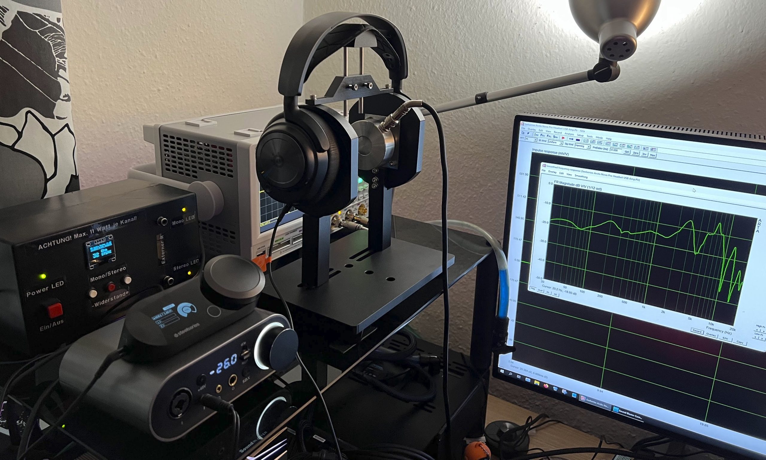
The complete measurement setup and methodology is described in detail in the article linked below. We can dispense with these redundant details. Nevertheless, it is recommended to have read this article at least once.

Finaler Testaufbau für den Test von Kopfhörern-und Headsets – Messen statt Schätzen und die Hintergründe

Important clue: The Harman curve

The so-called Harman curve is an (optimal) sound signature that most people prefer in their headphones. It is thus an accurate representation of how, for example, high-quality loudspeakers sound in an ideal room, and it shows the target frequency response of perfectly sounding headphones. Thus, it also explains which levels should be boosted and which should be attenuated based on this curve. This also explains the term “bathtub tuning”, which is often cited, but in which the Harman curve is completely overused and exaggerated.

For this reason, the Harman curve (also called the “Harman target”) is one of the best frequency response standards for enjoying music with headphones, because compared to the flat frequency response (neutral curve), the bass and treble are slightly boosted in the Harman curve. This “curve” was created and published in 2012 by a team of scientists led by sound engineer Sean Olive. At the time, the research also included extensive blind tests with different people testing different headphones. Based on what they then liked (or disliked), the researchers found and defined the most universally popular sound signature.

Headphone tuning can be really problematic because of the human anatomy. Everyone has a slightly different pinna and ear canal, which affects how individuals perceive certain frequencies. In extreme cases, there is a few dB difference from person to person, which then explains the small differences in some measurements with artificial ears. Furthermore, if the sound is not absorbed, it is additionally reflected by other surfaces. Theoretically, a torso could also be included in the test setup, but that would be far too time-consuming.

Measurement of the frequency response

Let’s now move on to the measurement, where the headset was operated in analog directly on the Creative Sound Blaster AE-9 as a reference (yellow curve) and then on the included USB DAC (light turquoise curve) for a better comparison. The output impedance of the power amplifier of the AE-9 is well below one ohm, so that especially in the bass range no impedance shifts and thus additional measurement errors arise. You can see the implied bathtub very nicely in both curves, but it weakens badly in the bass and is only more pronounced in the lower mids (200 to 250 Hz). Unfortunately, you get the dreaded cardboard sound, and I’m afraid that the somewhat too soft and uncontoured ear pads are also to blame for that. Insiders know this from the party basement, where cheap Chinese scratch boxes boom and drone.

In the bass range, the gap is also audible at around 70 Hz, while the level below increases again somewhat. I would have preferred to see the hump of the curve a little further to the right, but it is what it is. And yes, it is a gaming headset. The dark curve is the Harman target explained above, which is unfortunately missed by a wide margin. Linear also works differently. So much for the unsmoothed measurement result as curves.

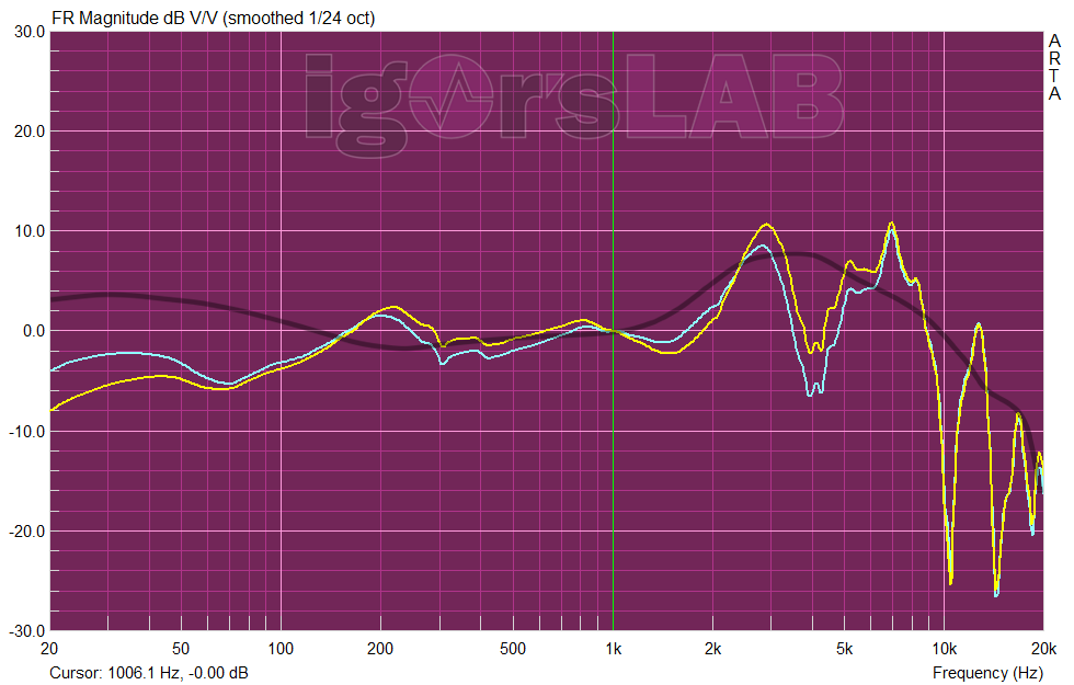
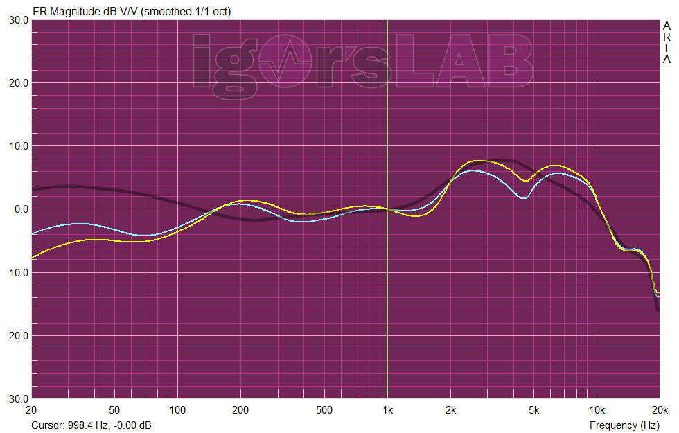
If you now smooth the whole thing down to the stop, the result is a somewhat rounder curve, which, however, fully confirms all points of criticism. The lower midrange is too dominant, while the bass remains in the background. The dip at about 70 Hz cannot be concealed acoustically. At 2.5 to 3 KHz, we see the aurally induced level rise, which is slightly different from the ideal line of the Harman curve. In addition, the drivers jitter in the super-tweeter at about 7 KHz, which drives the sibilants and blow-off noises of instruments into the metallic.

Cumulative spectra (CSD, SFT, Burst)

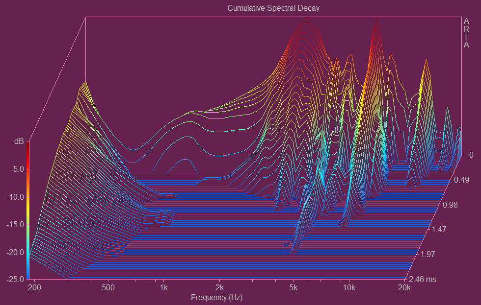
The cumulative spectrum refers to various types of graphs showing time-frequency characteristics of the signal. They are generated by sequentially applying the Fourier transform and appropriate windows to overlapping signal blocks. These analyses are based on the frequency response diagram already shown above, but additionally contain the element of time and now show very clearly as a 3D graphic (“waterfall”) how the frequency response develops over time after the input signal has been stopped. Colloquially, such a thing is also called “fading out” or “swinging out”. Normally, the driver should also stop as soon as possible after the input signal is removed. However, some frequencies (or even whole frequency ranges) will always decay slowly(er) and then continue to appear in this diagram as longer lasting frequencies on the time axis. From this, you can easily see where the driver has glaring weaknesses, perhaps even particularly “clangs” or where resonances occur in the worst case and could disturb the overall picture.

Cumulative Spectral Decay (CSD)
Cumulative spectral decay (CSD) uses the FFT and a modified rectangular window to analyze the spectral decay of the impulse response. It is mainly used to analyze the driver response. The CSD typically uses only a small FFT block shift (2-10 samples) to better visualize resonances throughout the frequency range, making it a useful tool for detecting resonances of the transducer. The picture shows very nicely the transient response and some present bass resonances in the upper bass and especially in the lower mids.

The cardboard sound and the overemphasis have to come from somewhere. The diaphragm resonates a bit badly below 400 Hz. Lousy, highly compressed MP3 files or lousy YouTube streams are forcibly crystallized by the extreme peaks in the high frequencies, but with very good recordings this is absolutely too much. You can love it or hate it. A matter of taste.

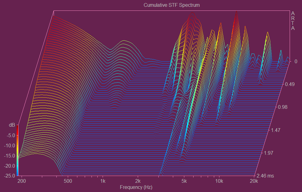
Short-time Fourier Transform (STF)
The Short-time Fourier Transform (STF) uses the FFT and Hanning window to analyze the time-varying spectrum of the recorded signals. Here, one generally uses a larger block shift (1/4 to 1/2 of the FFT length) to analyze a larger part of the time-varying signal spectrum, especially approaching application areas such as speech and music. In the STF spectrum we can now also see very nicely the work of the drivers, which afford various weaknesses in some frequency ranges. This “dragging” at the lower frequencies below 500 Hz is then repeated several times between about 2.5 and about 10 kHz. This is not really nice and it also confirms the measured frequency response.

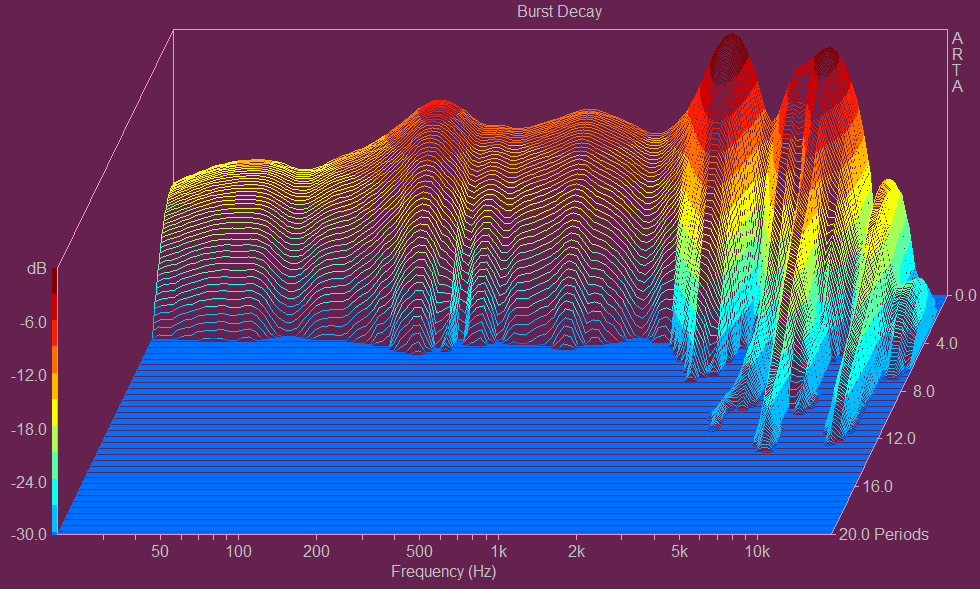
Burst Decay

In CSD, the plot is generated in the time domain (ms), while the burst decay plot used here is represented in periods (cycles). And while both methods have their advantages and disadvantages (or limitations), it’s fair to say that plotting in periods may well be more useful for determining the decay of a driver with a wide bandwidth. And that’s exactly where the headset also performs rather mediocrely. We see especially strong resonance vibrations in the high-frequency range again. This is probably supposed to sound especially “crispy”, but it also tugs at your nerves a bit when you want to listen to music. It is still okay for gaming, but the fun unfortunately stops for music.

Interim summary

With that, Igor’s part is (almost) already done and at least it hasn’t become a complete review. Only the warning not to overdo it with the upper bass and especially the lower mids. The USB DAC with the built-in sound solution produces sufficient levels and at least delivers better than any motherboard’s onboard solution. That’s on the credit side.

Microfontest

You can hear for yourself how the microphone performs here (Igor again). Note that the low cut already starts well above 100 Hz, so that especially the upper bass of Igor’s voice is completely missing and it sounds neither full nor authentic.

This test was performed on the reference AE-9, but the result on the included GameDAC Gen 2 turns out practically identical. With a bit of software gadgetry in Steelseries GG / Sonar, it might be possible to get more out of this, but the result is primarily one thing: quite quiet. Without increasing the volume afterwards, you will probably get lost in the voice chat quite quickly. Igor also had to use the Mic Boost fully to be heard and listened to.