


Test setup and basics
Now comes the moment of truth, once again. The test setup is final and the basis remains the familiar measurement microphone that has already proven itself for the in-ears. I found the suggestions for the realization at Oratory. In general, so-called couplers with clearly defined volumes and built-in, properly calibrated measurement microphones are used to measure the transmission behavior of headphones. The rest is then also based on the object to be measured.
The setup can be used just as well for plug-in headphones (in-ears) and small headphones (e.g. from hearing aids) as for simpler headphones and headsets as so-called on-ears (headphones with supraaural cushions). For such headphones (on-ear), the “artificial ear” according to IEC 318 is useful, which I have now followed with the implementation. I also use the Creative AE-9 as a sound card, to which the measurement microphone is connected with a sufficiently low noise level. As an output, I use a HIFIMAN EF400 to control the headphones, as this is possible via an analog jack.
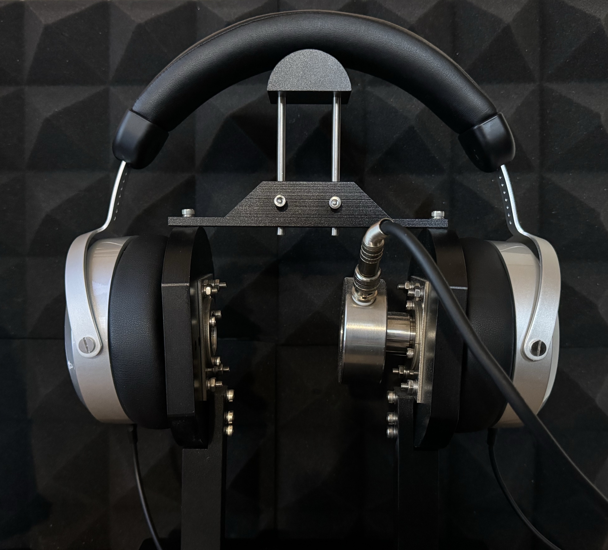
The thick over-ears, i.e. circumaural or ear-enclosing headphones, are not easy to handle when it comes to measurement and, above all, reproducibility. This is because there are not yet any truly standardized couplers. The reasons for this lie in the difficulties of measurement technology and the many influencing factors that make reliable reproducibility almost impossible. Therefore, such circumaural headphones are mainly measured with appropriately modified couplers for supraaural headphones by using an additional flat plate as a support for the circumaural cushion (see picture above).
An important reference point for headphones: the Harman curve
The so-called Harman curve is an (optimal) sound signature that most people prefer in their headphones. It is therefore an accurate representation of how, for example, high-quality speakers sound in an ideal room and it shows the target frequency response of perfect sounding headphones. It also explains which levels should be boosted and which should be attenuated when using this curve as a basis. This also explains the term “bathtub tuning”, which is often quoted, but in which the Harman curve is completely misused and exaggerated.
For this reason, the Harman curve (also known as the “Harman target”) is one of the best frequency response standards for enjoying music with headphones, because compared to the flat frequency response (neutral curve), the bass and treble are slightly boosted in the Harman curve. This “curve” was created and published in 2012 by a team of scientists led by sound engineer Sean Olive. The research at the time included extensive blind tests with different people testing different headphones. Based on what they liked (or didn’t like), the researchers found and defined the most popular sound signature.
Tuning headphones can be really problematic due to the human anatomy. Everyone has a slightly different pinna and ear canal, which affects how individuals perceive certain frequencies. In extreme cases, there is a difference of a few dB from person to person, which explains the small differences in some measurements with artificial ears. Furthermore, if the sound is not absorbed, it is also reflected by other surfaces. Theoretically, a torso could also be included in the test setup, but that would be far too time-consuming.
Frequency response
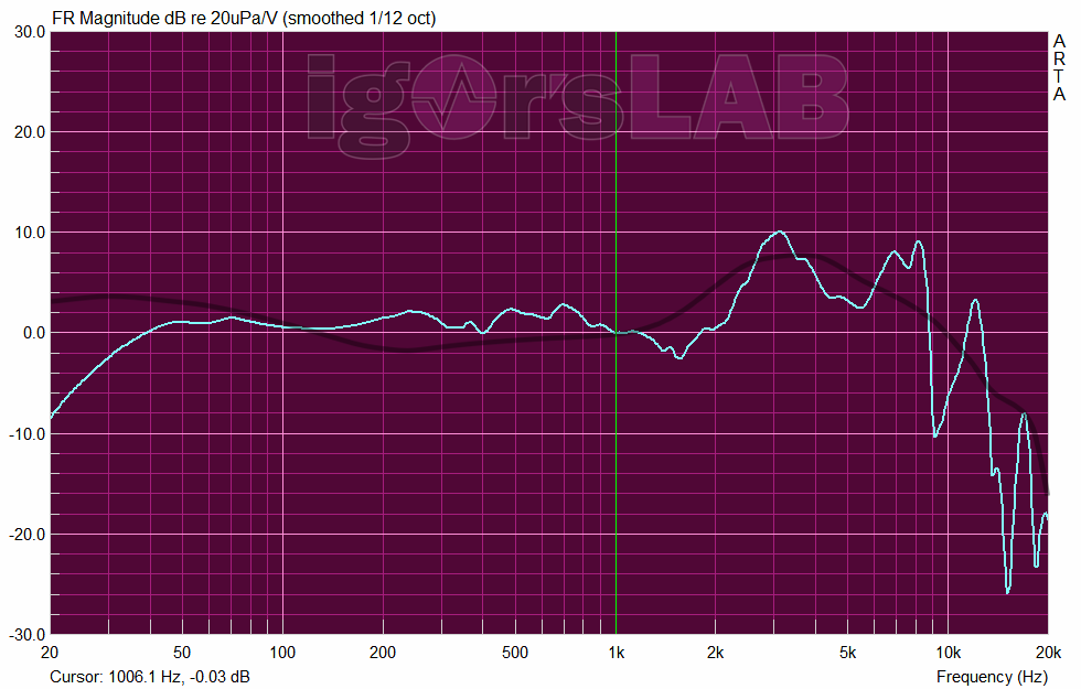
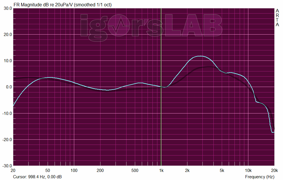
The Harman curve just mentioned is shown as a dark line in the diagram. Let us first evaluate the unsmoothed measurement. If we superimpose the light blue curve (HiFiMAN HE400se) and the black curve (Harman), interesting findings emerge. The output impedance of the HiFiMAN EF400 is virtually zero, so that a slight mismatch due to excessive impedance can be ruled out. In the high frequency range, the peak is at around 3 KHz and at 3 to 7 KHz, after which the curve drops off again.
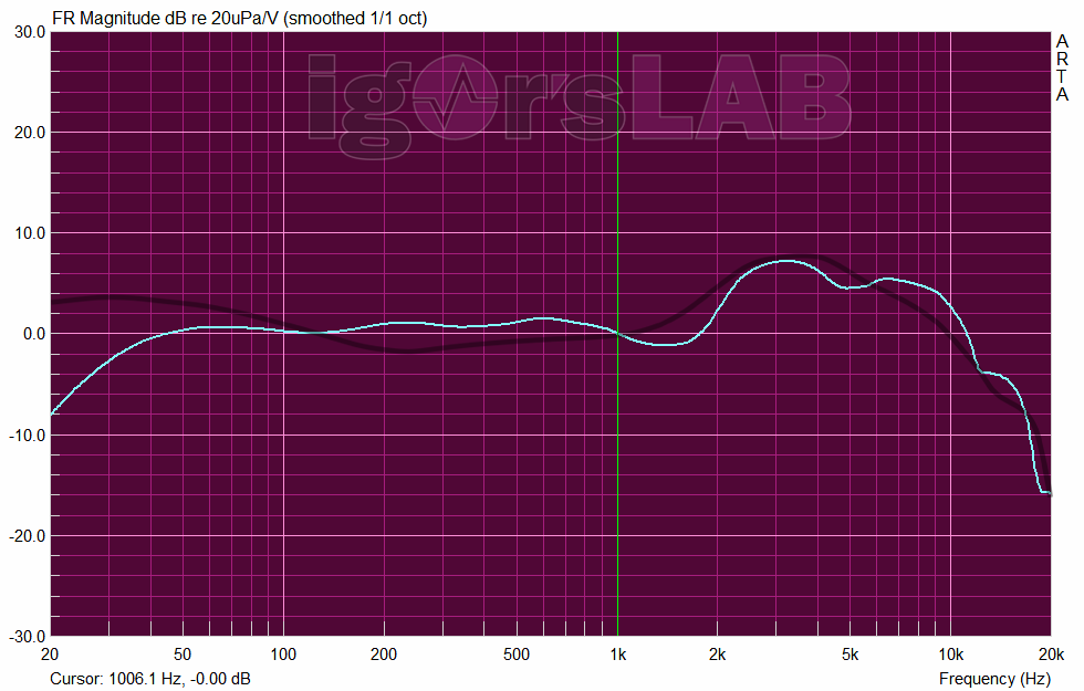
If you smooth out the curves, the whole thing definitely doesn’t look like a bathtub. The mids are slightly boosted, below 40 Hz the bass drop-off is of course due to the system and design. Nevertheless, there is enough low bass and the level stability is almost epic if you have a good amplifier. Here, too, we see the slight high-frequency exaggeration, but this can be eliminated quite easily with a parametric equalizer (see tutorial).
Parametric equalizer
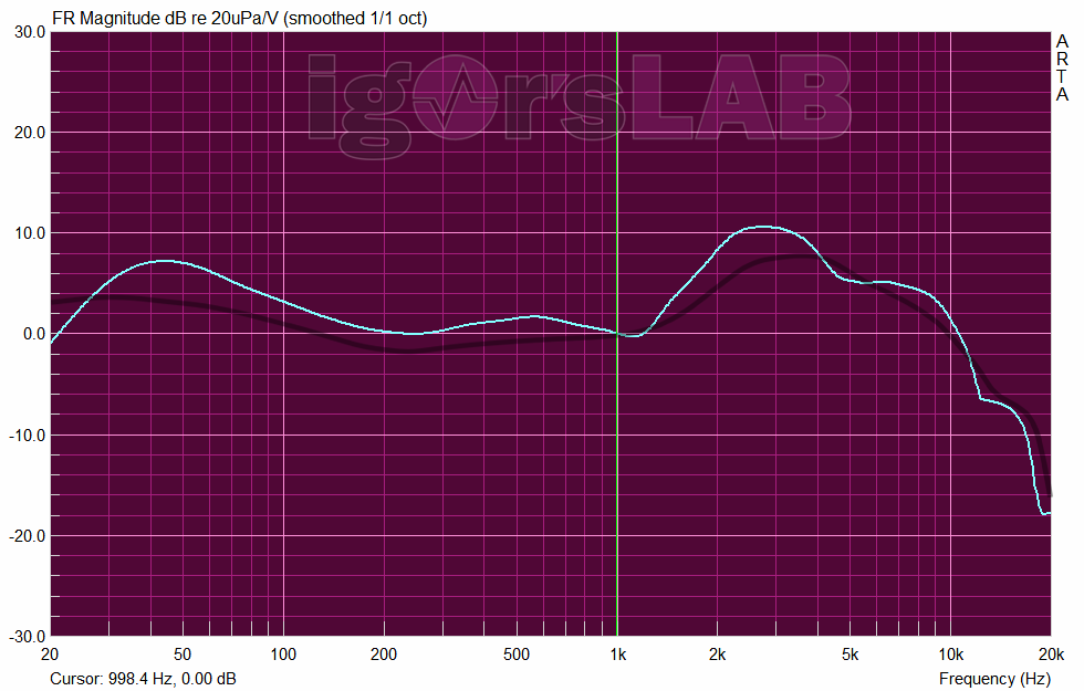
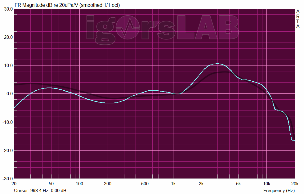
As I wrote in detail in the tutorial on the APU and PEACE equalizers, you can also use the stored profiles with AutoEQ. There are even three for the HIFIMAN HE400se, one each from Crinacle, RTINGS and Oratory. The frequency ranges used are similar, it’s just a matter of interpreting the filter and the level, as all three had slightly different measurement results. Our curve was amazingly similar to that of RTINGS, so I would also use this profile. But such things are very subjective and are therefore up to you. This is what the curves look like with the EQ profile activated:
Cumulative spectra
The cumulative spectrum refers to different types of diagrams that show the time-frequency characteristics of the signal. They are generated by successively applying the Fourier transform and suitable windows to overlapping signal blocks. These analyses are based on the frequency response diagram shown above, but also contain the time element and now show very clearly as a 3D graphic (“waterfall”) how the frequency response develops over time after the input signal has been stopped. Colloquially, this is also known as “decay” or “decay”. Normally, the driver should also stop as quickly as possible after the input signal has ceased. However, some frequencies (or even entire frequency ranges) will always decay slowly(er) and then continue to appear in this diagram as longer-lasting frequencies on the time axis. This makes it easy to recognize where the driver has glaring weaknesses, perhaps even particularly “clattery” or where, in the worst case, resonances could occur and disturb the overall picture.
Burst decay
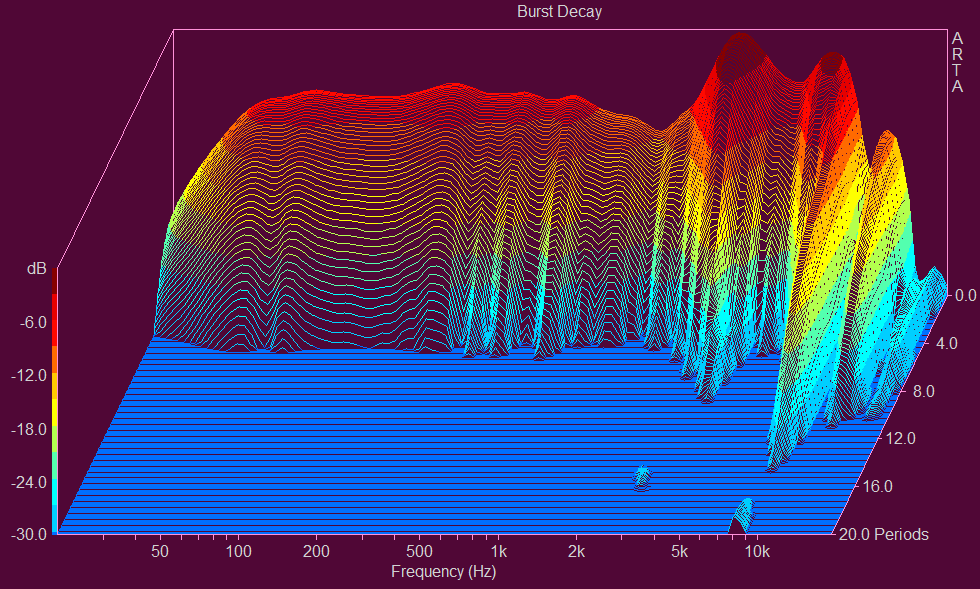
The “burst decay” refers to the gradual fading or decay of a signal or wave after a sudden impulse or “burst”. Such a burst can be caused by a sudden injection of energy, for example, and the subsequent decay describes the way in which the system returns to its initial state. The burst decay is used in the context of analyzing signals in audio processing. It is important to understand burst decay as it can affect the performance and quality of a system. In audio engineering, for example, burst decay can cause distortion or unwanted noise if it is not properly controlled.
Here, it is the engineer’s job to design systems that minimize such interference and handle burst decay effectively. With CSD, the plot is generated in the time domain (ms), whereas the burst decay plot used here is plotted in periods (cycles). And while both methods have their advantages and disadvantages (or limitations), it is fair to say that plotting in periods can be more useful for determining the decay of a driver with a wide bandwidth. The magnetostat does an almost perfect job here, you can leave it at that. There is not much resonance, only in the treble. Bass and mids are absolutely clean.
STFT
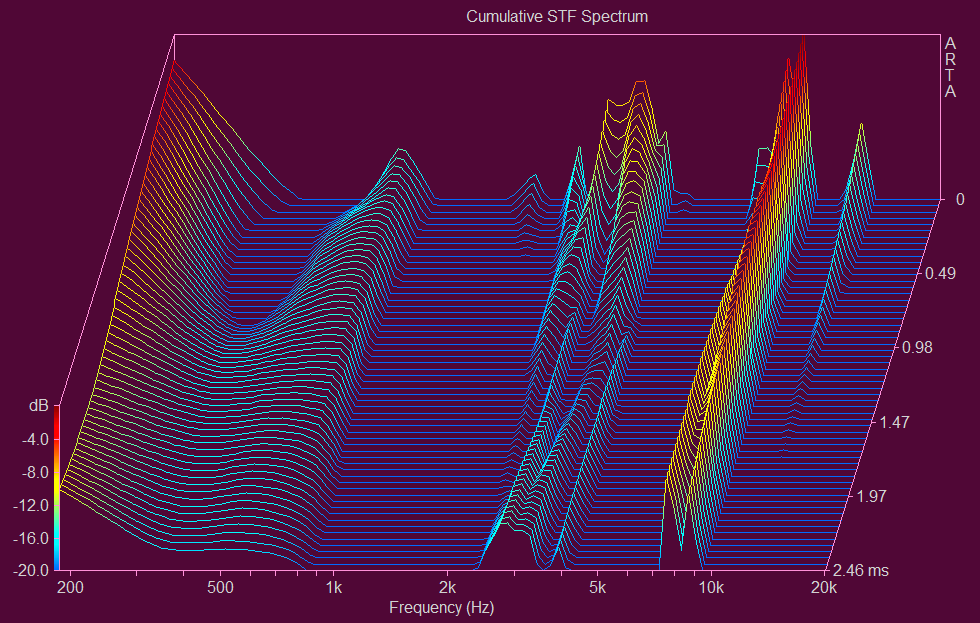
The Short-Time Fourier Transform (STFT) is a method for time-frequency analysis of signals in audio technology. In terms of headphone measurements, the STFT is particularly useful for investigating how the frequency content of a signal changes over time. Traditional Fourier transforms allow a signal to be broken down into its frequency components, but do not provide information about when these components occur in the signal. This can be a problem when working with signals that change over time, such as music or speech. This is where the STFT comes in, using the FFT and Hanning window to analyze the time-varying spectrum of the recorded signals.
The STFT divides a longer signal into smaller segments and performs a Fourier transformation for each of these segments. This allows us to see how the frequencies vary over time. So in terms of headphone measurement, the STFT allows us to see how the frequency response of a headphone changes over time, which can provide valuable insight into its performance and sound quality. It is important to note that the choice of segment length in the STFT is a compromise: with longer segments we get more accurate frequency resolution, but lose temporal resolution.
With shorter segments, it is exactly the opposite: we get a higher temporal resolution but lose frequency resolution. Therefore, the size of the segments must be chosen carefully to achieve the best possible results. The STFT is therefore a very powerful tool for analyzing audio signals and assessing the performance of audio devices such as headphones. Once again, the headphone performs quite well and the membrane does what is expected of it. However, we can see real resonances here, especially in the high frequency peaks, which generate a slightly higher level than the actual electrical power applied. As you can see, in the end you need all the diagrams to make an objective judgment. Burst decay alone is not quite enough.


157 Antworten
Kommentar
Lade neue Kommentare
Veteran
Urgestein
Urgestein
Veteran
1
Urgestein
Urgestein
1
Veteran
Urgestein
1
Veteran
Mitglied
Mitglied
Urgestein
Mitglied
Veteran
Mitglied
Alle Kommentare lesen unter igor´sLAB Community →